

✍️ Week 1 lesson 6 of DataTalksClub 2022 data engineering zoomcamp, reviewing 💽 SQL basics with the 🚕 NYC taxi trips data
Today, we will follow DataTalksClub's video: DE Zoomcamp 1.2.6 - SQL Refreshser.
Which is part of the DataTalksClub 2022 Data engineering Zoomcamp week 1 repo.
In our last post, we learned how to build containers with Docker Compose, following DataTalksClub's video: DE Zoomcamp 1.2.5 - Running Postgres and pgAdmin with Docker-Compose.

💬 In this lesson, we will flex our SQL muscles 💪 while exploring the NYC taxi trip data. For this, we will:
- Ingest the taxi zone lookup file from the NYC taxi trips into our ny_taxi database.
- Review the SQL basics:
2.1 Write inner joins with the WHERE and JOIN clauses.
2.2 Verify that these queries are equivalent.
2.3 Use CONCAT to combine string type columns.
2.4 Find missing data in both tables.
2.5 Delete a row in a table.
2.6 Frame joins as set operations.
2.7 Use a left join to find missing zones in the NYC taxi trips table.
2.8 Use a right join to find matches to a given location ID.
2.9 Use an outer join to find rows without a match on either table.
2.10 Group the NYC taxi trips table by dropoff day and summarize the fare and passenger count columns.
This post is part of a series. Find all the other related posts here

🏙️ Ingesting the taxi zone lookup file
We encountered the taxi zone lookup table when we first described the NYC taxi trip data. This file contains the mapping from the codes in the pickup (PULocationID) and dropoff (DOLocationID) columns in the trips data to names an NYC street aware human can relate to.
Let's return to our upload-data.ipynb and add cells at the bottom of the file to download the taxi zone lookup table and insert it on the ny_taxi database under a new table (zones).
import subprocess

URL = "https://s3.amazonaws.com/nyc-tlc/misc/taxi+_zone_lookup.csv"
csv_name = "taxi+_zone_lookup.csv"

# download the csv
proc = subprocess.run([
    "wget",
    URL,
    "-O",
    csv_name,
])
assert proc.returncode == 0, (URL, proc.returncode)If the download process went well, there should be a file named taxi+_zone_lookup.csv in our working directory. Let's read it with Pandas.
import pandas as pd
# read file
zone_lookup = pd.read_csv(csv_name)
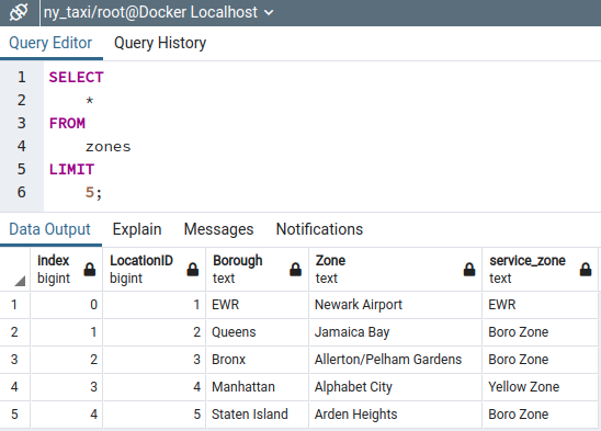
zone_lookup.head()which should print a table like this
| LocationID | Borough | Zone | service_zone | |
|---|---|---|---|---|
| 0 | 1 | EWR | Newark Airport | EWR |
| 1 | 2 | Queens | Jamaica Bay | Boro Zone |
| 2 | 3 | Bronx | Allerton/Pelham Gardens | Boro Zone |
| 3 | 4 | Manhattan | Alphabet City | Yellow Zone |
| 4 | 5 | Staten Island | Arden Heights | Boro Zone |
So LocationID 2 is Queens 👑. Got it!
Let's create a table in the ny_city database, call it zones and insert the data in the zones lookup file
from sqlalchemy import create_engine

# DB connection engine
engine = create_engine('postgresql://root:root@localhost:5432/ny_taxi')

zone_lookup.to_sql(name='zones', con=engine, if_exists='replace')
To check if the data was inserted, let's open a web browser tab pointing to pgAdmin (localhost:8080), create and configure the server, and use the query tool to find the data in our new zones table.
📖 SQL basics review
We want to start getting comfortable with SQL by creating simple queries that we can use in future lessons. First, let's check the data in the NYC taxi trips table.
SELECT
	"tpep_pickup_datetime",
	"tpep_dropoff_datetime",
	"PULocationID",
	"DOLocationID"
FROM
	yellow_taxi_data
LIMIT
	5;
Note that the selected column names are in quotes since some use capital letters. This query should return the first five records in the NYC taxi trips table.
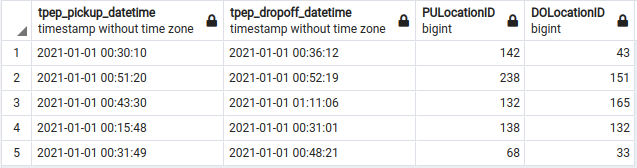
Also, note in the returned table that the PULocationID (pickup location ID) and DOLocationID (dropoff location ID) refer to the LocationID column in the zones table. Let's combine the NYC taxi trips and zones tables so that we can see each taxi trip's pickup and dropoff location information, not just the IDs.
🧘 Inner join: Zones in the NYC taxi trips
There are a couple of ways to write the SQL query that combines the two tables in the way we expect it. The critical thing to remember is that we are trying to use the IDs in two different columns in the yellow_taxi_data table, i.e., for pickup and dropoff locations, so our query will do the same thing twice.
First, let's write the query using a WHERE clause.
SELECT
	"tpep_pickup_datetime",
	"tpep_dropoff_datetime",
	"total_amount",
	zpu."Borough" AS "zpu_borough",
	zpu."Zone"  AS "zpu_zone",
	zdo."Borough" AS "zdo_borough",
	zdo."Zone"  AS "zdo_zone"
FROM
	yellow_taxi_data t,
	zones zpu,
	zones zdo
WHERE
	t."PULocationID" = zpu."LocationID" AND
	t."DOLocationID" = zdo."LocationID"
ORDER BY
	"tpep_pickup_datetime" ASC
LIMIT
	5;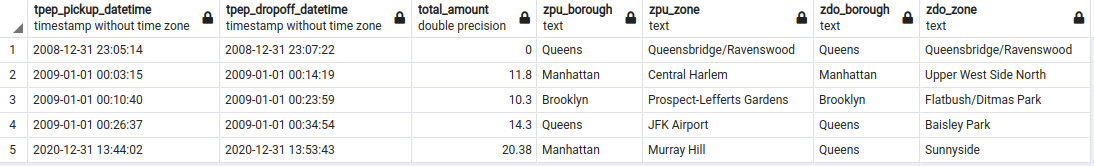
Note that we have three tables in the FROM statement: The yellow_taxi_data table aliased as t, the zones table aliased as zpu (zone pickup), and again the zones table but this time aliased as zdo (zone dropoff). Also, note that in the SELECT statement, the last four lines refer to fields (columns) in the zones table, the first two in the aliased zpu, and the last two in the aliased zdo. In this way, we are asking the database engine to return the Borough and Zone columns for pickup and dropoff locations.
The magic happens in the WHERE clause. Typically, we use the WHERE clause to filter records in a table, but this query effectively matches the records in the yellow_taxi_data table with their counterparts in the zones table, based on the location ID. As stated before, we need to write this pairing twice, once for the pickup column and once for the dropoff column.
Show me the records in the yellow_taxi_data table,
where the pickup location ID value exists
in the zones table location ID column, and
where the dropoff location ID value exists
in the zone table location ID column.
-Excerpt translation from the query using WHERE
Another way of writing this query is using the JOIN statement.
SELECT
	"tpep_pickup_datetime",
	"tpep_dropoff_datetime",
	"total_amount",
	zpu."Borough" AS "zpu_borough",
	zpu."Zone"  AS "zpu_zone",
	zdo."Borough" AS "zdo_borough",
	zdo."Zone"  AS "zdo_zone"
FROM
	yellow_taxi_data t JOIN zones zpu
	    ON t."PULocationID" = zpu."LocationID"
	JOIN zones zdo
	    ON t."DOLocationID" = zdo."LocationID"
ORDER BY
	"tpep_pickup_datetime" ASC
LIMIT
	5;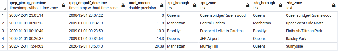
As you can see, the data output using JOIN is equivalent to that when using WHERE. In this case, we don't need to use the WHERE clause since the ON operator takes care of combining the yellow_taxi_data and zones table based on the location ID. Note that we have to do two join operations, one for pickups and one for dropoff.
Join the yellow_taxi_data and zones table on the pickup location ID,
and then,
join the result with the zones table on the dropoff location ID.
-Excerpt translation from the query using JOIN
🕳️ Down the DataFrames equality rabbit hole
We asserted that the two ways of writing the SQL queries, i.e., using JOIN and using WHERE, returned the same data output. We can verify this by looking at the respective data output tables in the figures above, but these have been limited to the first five returned rows. But, would this assertion hold for all the returned records? Being the first time making this comparison, I'd say trust but verify. In the last section, we did the trusting, and now we will do the verifying.
A simple way to go about this is to edit the SQL queries to sort the data output by all the fields, so if the data outputs are indeed the same but unsorted, we first sort them and then compare them using Pandas. Let's return to our upload-data.ipynb and add cells at the bottom of the file to compare the data output.
sql_where = '''
SELECT
	"tpep_pickup_datetime",
	"tpep_dropoff_datetime",
	"total_amount",
	zpu."Borough" AS "zpu_borough",
	zpu."Zone"  AS "zpu_zone",
	zdo."Borough" AS "zdo_borough",
	zdo."Zone"  AS "zdo_zone"
FROM
	yellow_taxi_data t,
	zones zpu,
	zones zdo
WHERE
	t."PULocationID" = zpu."LocationID" AND
	t."DOLocationID" = zdo."LocationID"
ORDER BY
	"tpep_pickup_datetime" ASC,
	"tpep_dropoff_datetime" ASC,
	"total_amount" ASC,
	"zpu_borough" ASC,
	"zpu_zone" ASC,
	"zdo_borough" ASC,
	"zdo_zone" ASC;
'''sql_join = '''
SELECT
"tpep_pickup_datetime",
"tpep_dropoff_datetime",
"total_amount",
zpu."Borough" AS "zpu_borough",
zpu."Zone" AS "zpu_zone",
zdo."Borough" AS "zdo_borough",
zdo."Zone" AS "zdo_zone"
FROM
yellow_taxi_data t JOIN zones zpu
ON t."PULocationID" = zpu."LocationID"
JOIN zones zdo
ON t."DOLocationID" = zdo."LocationID"
ORDER BY
"tpep_pickup_datetime" ASC,
"tpep_dropoff_datetime" ASC,
"total_amount" ASC,
"zpu_borough" ASC,
"zpu_zone" ASC,
"zdo_borough" ASC,
"zdo_zone" ASC;
'''Since we already have Pandas imported and the SQLAlchemy connection engine running, we can just load the data outputs to DataFrames and use the equality check method.
where_df = pd.read_sql_query(sql_where, con=engine)
join_df = pd.read_sql_query(sql_join, con=engine)
print(where_df.equals(join_df))
The last instruction in the code snippet above should print True, which settles the matter, announcing we have reached the end of the rabbit hole 🐰.
🔀 Combining selected columns
Going back to our limited WHERE SQL query, remember we had two columns (borough and zone) for pickups and the same two columns for dropoffs. Let's combine them to simplify the data output using SQL's CONCAT function.
SELECT
	"tpep_pickup_datetime",
	"tpep_dropoff_datetime",
	"total_amount",
	CONCAT(zpu."Borough", ' / ', zpu."Zone") AS "pickup_loc",
	CONCAT(zdo."Borough", ' / ', zdo."Zone") AS "dropoff_loc"
FROM
	yellow_taxi_data t,
	zones zpu,
	zones zdo
WHERE
	t."PULocationID" = zpu."LocationID" AND
	t."DOLocationID" = zdo."LocationID"
ORDER BY
	"tpep_pickup_datetime" ASC
LIMIT
	5;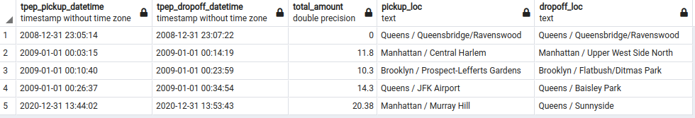
🔎 Finding missing pickup or dropoff locations
Let's check if there are any missing pickup or dropoff locations in the yellow_taxi_data.
SELECT
	"tpep_pickup_datetime",
	"tpep_dropoff_datetime",
	"total_amount",
	"PULocationID",
	"DOLocationID"
FROM
	yellow_taxi_data t
WHERE
	t."PULocationID" is NULL OR
	t."DOLocationID" is NULL
ORDER BY
	"tpep_pickup_datetime" ASC
LIMIT
	5;
This query returns an empty data output, indicating that there are no NULL pickup or dropoff locations in the yellow_taxi_data table.
Now let's check if all the pickup and dropoff location IDs in the yellow_taxi_data table are accounted for in the zones table location ID.
SELECT
	"tpep_pickup_datetime",
	"tpep_dropoff_datetime",
	"total_amount",
	"PULocationID",
	"DOLocationID"
FROM
	yellow_taxi_data t
WHERE
	t."PULocationID" NOT IN (SELECT "LocationID" FROM zones) OR
	t."DOLocationID" NOT IN (SELECT "LocationID" FROM zones)
ORDER BY
	"tpep_pickup_datetime" ASC
LIMIT
	5;
Again, we got an empty data output. This hints at the possibility that these data quality aspects were checked and fixed by the data providers before sharing the data, which is excellent for real work, but not so much for teaching table joins 😉.
☠️ Deleting a row in a table
For illustration purposes, let's remove one row from the zones table. We will run a simple query on the yellow_taxi_data table to decide which row to remove.
SELECT
	"tpep_pickup_datetime",
	"tpep_dropoff_datetime",
	"PULocationID",
	zones."Zone"
FROM
	yellow_taxi_data t JOIN zones
		ON t."PULocationID" = zones."LocationID"
LIMIT
	1;
It looks like we have a volunteer! Let's create a query to delete it from the zones table.
DELETE FROM zones WHERE "LocationID" = 142;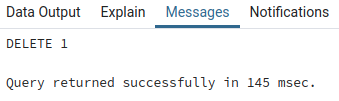
Now let's re-run the query above that checks if all the pickup and dropoff location IDs in the yellow_taxi_data table are accounted for in the zones table location ID.
SELECT
	"tpep_pickup_datetime",
	"tpep_dropoff_datetime",
	"total_amount",
	"PULocationID",
	"DOLocationID"
FROM
	yellow_taxi_data t
WHERE
	t."PULocationID" NOT IN (SELECT "LocationID" FROM zones) OR
	t."DOLocationID" NOT IN (SELECT "LocationID" FROM zones)
ORDER BY
	"tpep_pickup_datetime" ASC
LIMIT
	5;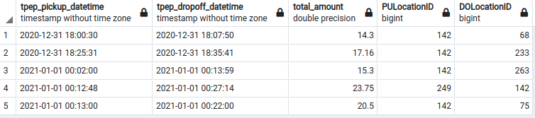
Note that the returned records have a 142 value in the PULocationID or DOLocationID columns.
Also, if we re-run the JOIN query we used to find the location ID to be deleted, we will get a different data output.
SELECT
	"tpep_pickup_datetime",
	"tpep_dropoff_datetime",
	"PULocationID",
	zones."Zone"
FROM
	yellow_taxi_data t JOIN zones
		ON t."PULocationID" = zones."LocationID"
LIMIT
	1;
The reason for this is that this kind of table join (inner join) will only return the records that match the ON condition, i.e., where the yellow_taxi_data table PULocationID values are equal to the values in the zones table LocationID column. Effectively, the inner join returns the records at the intersection (set operation) of location ID values in the two tables.
🎱 Joins are set operations
Vaidehi Joshi (2017) explains the connection between set operations and SQL joins in the post: Set Theory: the Method To Database Madness. There, you will find a figure from C.L. Moffatt's visual representation of SQL joins that neatly explains what data output we should expect from each join operation.
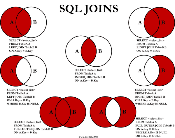
Ours is the INNER JOIN case (middle center). Note that we didn't add the INNER modifier as this is the default behavior. Also, in our last query, we limited the output to one record, but if we hadn't, the data output would have been all the records in the yellow_taxi_data and zones table that share location IDs (intersection).
⬅️ Left join: Missing zones in NYC taxi trips
We use left joins when we would like to show all the records in the left table, i.e., the first table in the FROM section of the query, augmented with information in another table (the right table), based on the matching condition expressed after the ON operator. When there is no record in the right table with the requested joining value, return the selected information in the left table, adding a missing flag in the right table selected columns. Left joins are represented in the upper left diagram in C. L. Moffatt's figure.
To illustrate the LEFT JOIN syntax, let's modify our original inner join query (before we used the CONCAT function).
SELECT
	"tpep_pickup_datetime",
	"tpep_dropoff_datetime",
	"total_amount",
	zpu."Borough" AS "zpu_borough",
	zpu."Zone"  AS "zpu_zone",
	zdo."Borough" AS "zdo_borough",
	zdo."Zone"  AS "zdo_zone"
FROM
	yellow_taxi_data t LEFT JOIN zones zpu
	    ON t."PULocationID" = zpu."LocationID"
	LEFT JOIN zones zdo
	    ON t."DOLocationID" = zdo."LocationID"
WHERE
	t."PULocationID" = 142 OR
	t."DOLocationID" = 142
ORDER BY
	"tpep_pickup_datetime" ASC
LIMIT
	5;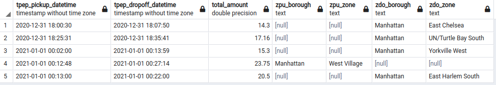
Note that all the records from the yellow_taxi_data are returned, even those without a match in the zones table.
Show me ALL the records in the yellow_taxi_data table,
and their corresponding data in the zones table,
but if they have none,
just show me null.
-Excerpt translation from the LEFT JOIN query
➡️ Right join: One zone to many NYC taxi trips
The top right diagram in C. L. Moffatt's figure represents a right join. These are created with the RIGHT JOIN statement, and as you can probably tell, most of the time, we can write them as equivalent left joins. So why bother learning about them?
The main reason is a practical rule where in many-to-one table relationships, we think of the table with the "many" records as the left table, and the one with the unique records (to-one) as the right table. This is an arbitrary decision and, most of the time, an unwritten rule, but it helps with consistency. In fact, it is the implicit assumption we made when joining the yellow_taxi_data and zones tables, i.e., the many locations in the yellow_taxi_table correspond to one location in the zones table.
Let's return to our previous query where we used left joins, adjust it to use right joins, and show the location ID values.
SELECT
	"tpep_pickup_datetime",
	"tpep_dropoff_datetime",
	"total_amount",
	zpu."LocationID" AS "zpu_location_id",
	zpu."Borough" AS "zpu_borough",
	zpu."Zone"  AS "zpu_zone",
	zdo."LocationID" AS "zdo_location_id",
	zdo."Borough" AS "zdo_borough",
	zdo."Zone"  AS "zdo_zone"
FROM
	yellow_taxi_data t RIGHT JOIN zones zpu
	    ON t."PULocationID" = zpu."LocationID"
	RIGHT JOIN zones zdo
	    ON t."DOLocationID" = zdo."LocationID"
WHERE
	zpu."LocationID" = 265 -- Unknown, NA
ORDER BY
	"tpep_pickup_datetime" ASC
LIMIT
	5;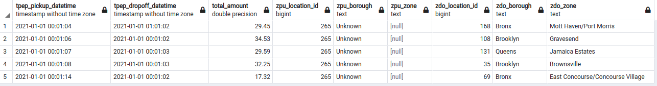
I restricted the query to show the match to pickup location 265 (borough: Unknown, zone: null). Note that the join operation finds the matching records in the yellow_taxi_data for every record in the zones table. As a result, we get a record in the data output for every match. If the joining keys are non-unique in the zones table, those duplicates will also get matched, so please consider this when designing your queries. This fact is true for any join, not just right joins.
🦦 Outer join: Show me all the things
The last join we will review is the full outer join, where all the records from both tables are returned. When there are no matching rows for the row in the left table, the right table columns will get a null value, and vice-versa. This case is represented by the bottom left diagram in C. L. Moffatt's figure above. Here, we will use the particular case where we are interested in learning which are the rows that didn't have a match (bottom right diagram), so we will restrict the output with a WHERE clause.
SELECT
	"tpep_pickup_datetime",
	"tpep_dropoff_datetime",
	"total_amount",
	t."PULocationID" AS "pu_location_id",
	zpu."LocationID" AS "zpu_location_id",
	zpu."Borough" AS "zpu_borough",
	zpu."Zone"  AS "zpu_zone"
FROM
	yellow_taxi_data t FULL OUTER JOIN zones zpu
	    ON t."PULocationID" = zpu."LocationID"
WHERE
    t."PULocationID" is NULL OR
    zpu."LocationID" is NULL
ORDER BY
	"tpep_pickup_datetime" ASC
LIMIT
	5;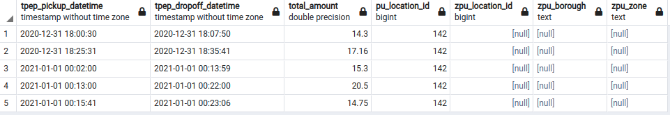
This result makes sense. We know that the location ID 142 is no longer in the zones table (we removed it!), so we see a sample of the left table (yellow_taxi_data) that didn't match on the zones table, as we did when we reviewed the left join clause.
🪣 Group by dropoff day
Let's look at the number of trips per day, using the dropoff date as the day to group by. We can use the DATE_TRUNC function to zero out the time component from the dropoff day timestamps in our query. Alternatively, we can cast the dropoff day timestamps as DATE type. Let's follow the latter approach, grouping by the newly cast date while using the COUNT aggregation function to count the records in each date group.
SELECT
	CAST(tpep_dropoff_datetime AS DATE) AS "day",
	COUNT(*) AS "dropoff_day_count"
FROM
	yellow_taxi_data t
GROUP BY
    "day"
ORDER BY
    "dropoff_day_count" DESC
LIMIT
    5;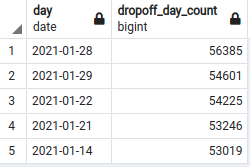
Neat! It looks like the 28 of January was exceptionally busy.
Now, what would be the largest fare paid on these days? or the maximum number of passengers?
SELECT
	CAST(tpep_dropoff_datetime AS DATE) AS "day",
	COUNT(*) AS "dropoff_day_count",
	MAX(total_amount) AS "max_total_amount",
	MAX(passenger_count) AS "passenger_count"
FROM
	yellow_taxi_data t
GROUP BY
    "day"
ORDER BY
    "dropoff_day_count" DESC
LIMIT
    5;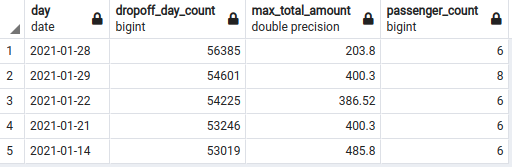
Cool! So it seems that, with luck, a driver can make $400 in a single trip. Also, what sort of vehicle sits eight passengers? I mean, most NYC yellow taxis (at least in the movies) can sit up to three people in the back seat. Weird!
Finally, imagine we would like to break down the data for each day by pickup location, perhaps to see when and where to send our drives to make the largest fare per trip.
SELECT
	CAST(tpep_dropoff_datetime AS DATE) AS "day",
	"PULocationID" AS "pickup_location",
	COUNT(*) AS "dropoff_day_count",
	MAX(total_amount) AS "max_total_amount",
	MAX(passenger_count) AS "passenger_count"
FROM
	yellow_taxi_data t
GROUP BY
	"day",
	"pickup_location"
ORDER BY
	"max_total_amount" DESC
LIMIT
    5;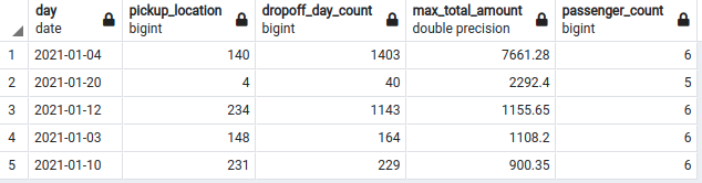
Zone 140 (Manhattan / Lenox Hill East) has the largest fare but lots of trips in a day (1403), so if the process is random, zone 4 (Manhattan / Alphabet city) represents a better option, with the second-largest fare in a day with only 40 trips. More work needs to be done to understand these trends, but we have accomplished reviewing the SQL knowledge we will need in future lessons.
📝 Summary
In this post we:
- Ingested the taxi zone lookup file from the NYC taxi trips into our ny_taxi database.
- Reviewed the SQL basics:
2.1 Wrote inner joins with the WHERE and JOIN clauses.
2.2 Verified that these queries are equivalent.
2.3 Used CONCAT to combine string type columns.
2.4 Found missing data in both tables.
2.5 Deleted a row in a table.
2.6 Understood joins as set operations.
2.7 Used a left join to find missing zones in the NYC taxi trips table.
2.8 Used a right join to find matches to a given location ID.
2.9 Used an outer join to find rows without a match on either table.
2.10 Grouped the NYC taxi trips table by dropoff day and summarized the fare and passenger count columns.

In our next lesson, we will set up our first project in the ☁️ Google Cloud Platform, create and configure a service account, and install gcloud CLI in our local machine.
